Loading EIS Data

AutoEIS requires two 1D arrays as input:

• ``freq``: Frequency array in Hz (np.ndarray[float])

• ``Z``: Complex impedance array in Ohms (np.ndarray[complex])

Both arrays must have the same length. The impedance follows the convention where the imaginary part is typically negative for capacitive behavior.

This notebook demonstrates how to load EIS data from various sources, including built-in datasets and instrument-specific file formats.

import autoeis as ae
ae.visualization.set_plot_style()

Built-in datasets

AutoEIS ships with two built-in datasets for testing and demonstration:

• ae.io.load_test_dataset() - a single EIS measurement

• ae.io.load_battery_dataset() - multiple EIS measurements from a battery cell during cycling

Both accept optional preprocess and noise arguments.

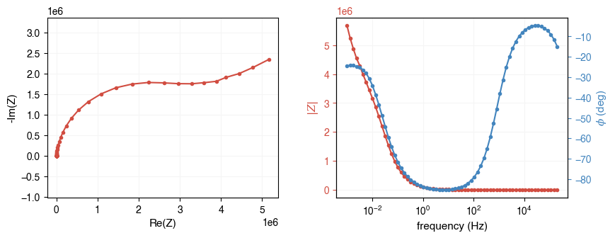
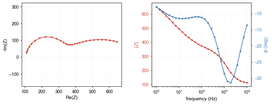
freq, Z = ae.io.load_test_dataset()
print(f"freq: shape={freq.shape}, dtype={freq.dtype}")
print(f"Z:    shape={Z.shape}, dtype={Z.dtype}")
ae.visualization.plot_impedance_combo(freq, Z)

freq: shape=(67,), dtype=float64
Z:    shape=(67,), dtype=complex128

array([<Axes: xlabel='Re(Z)', ylabel='-Im(Z)'>,
       <Axes: xlabel='frequency (Hz)', ylabel='$|Z|$'>,
       <Axes: ylabel='$\\phi$ (deg)'>], dtype=object)

Loading from instrument files

AutoEIS can load EIS data directly from proprietary instrument file formats using ae.io.load_eis_data(). This function combines two backends to support a wide range of instruments:

Instrument	File extension	instrument parameter
Gamry	.DTA	"gamry"
BioLogic	.mpt	"biologic"
ZPlot/ZView	.z	"zplot"
Autolab	.txt	"autolab"
Parstat	.txt	"parstat"
VersaStudio	.par	"versastudio"
PowerSuite	.txt	"powersuite"
CH Instruments	.txt	"chinstruments"
Eco Chemie	.dfr	"ecochemie"
Ivium	.idf, .ids	"ivium"
PalmSens	.pssession	"palmsens"
Spreadsheets	.xlsx, .ods	"spreadsheet"
CSV	.csv	None (auto-detected)

For formats with unique file extensions (e.g., .DTA, .mpt, .z), the instrument type is auto-detected. For formats that share extensions (e.g., .txt), you must specify the instrument parameter.

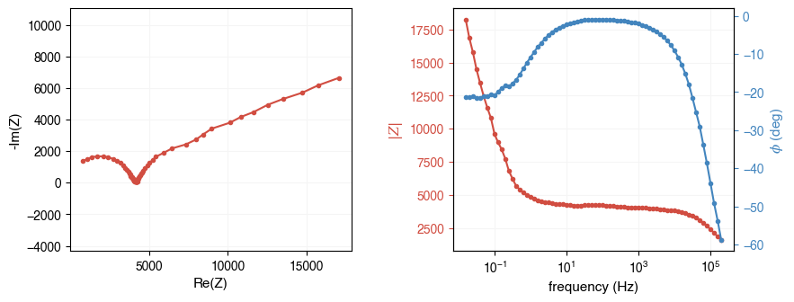
# Load from a Gamry .DTA file (auto-detected from extension)
fpath = ae.io.get_assets_path() / "exampleDataGamry.DTA"
freq, Z = ae.io.load_eis_data(fpath)
ae.visualization.plot_impedance_combo(freq, Z)

array([<Axes: xlabel='Re(Z)', ylabel='-Im(Z)'>,
       <Axes: xlabel='frequency (Hz)', ylabel='$|Z|$'>,
       <Axes: ylabel='$\\phi$ (deg)'>], dtype=object)

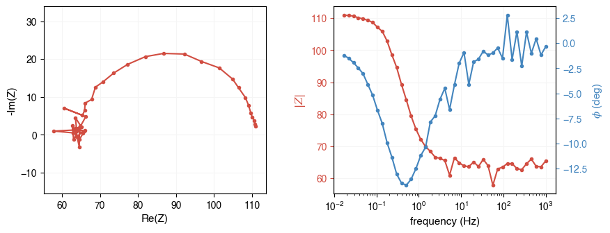
# Load from a BioLogic .mpt file (auto-detected from extension)
fpath = ae.io.get_assets_path() / "exampleDataBioLogic.mpt"
freq, Z = ae.io.load_eis_data(fpath)
ae.visualization.plot_impedance_combo(freq, Z)

array([<Axes: xlabel='Re(Z)', ylabel='-Im(Z)'>,
       <Axes: xlabel='frequency (Hz)', ylabel='$|Z|$'>,
       <Axes: ylabel='$\\phi$ (deg)'>], dtype=object)

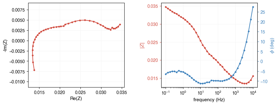
# For .txt formats, specify the instrument explicitly
fpath = ae.io.get_assets_path() / "exampleDataAutolab.txt"
freq, Z = ae.io.load_eis_data(fpath, instrument="autolab")
ae.visualization.plot_impedance_combo(freq, Z)

array([<Axes: xlabel='Re(Z)', ylabel='-Im(Z)'>,
       <Axes: xlabel='frequency (Hz)', ylabel='$|Z|$'>,
       <Axes: ylabel='$\\phi$ (deg)'>], dtype=object)

# Load from an Eco Chemie .dfr file (via pyimpspec backend)
fpath = ae.io.get_assets_path() / "data.dfr"
freq, Z = ae.io.load_eis_data(fpath, instrument="ecochemie")
ae.visualization.plot_impedance_combo(freq, Z)

array([<Axes: xlabel='Re(Z)', ylabel='-Im(Z)'>,
       <Axes: xlabel='frequency (Hz)', ylabel='$|Z|$'>,
       <Axes: ylabel='$\\phi$ (deg)'>], dtype=object)

Loading from generic formats

If your data is in a generic format (CSV, text, NumPy, etc.), you can load it directly with standard Python libraries and construct the freq and Z arrays yourself:

import numpy as np
import pandas as pd

# From a CSV with columns: frequency, Re(Z), Im(Z)
df = pd.read_csv("my_data.csv")
freq = df["frequency"].values
Z = df["Re(Z)"].values + 1j * df["Im(Z)"].values

# From a text file with columns: freq, Re(Z), -Im(Z)
freq, Zre, Zim_neg = np.loadtxt("my_data.txt", unpack=True)
Z = Zre - 1j * Zim_neg

Pay attention to the sign convention: some instruments store -Im(Z) instead of Im(Z). AutoEIS expects the standard complex impedance where the imaginary part is negative for capacitive behavior.